Numerical methods
Suppose that we dispose of a high-fidelity model (HFM) – or high-dimensional model (HDM), \(\mathcal{H}\), that depends on a given variability \(\mu\). We are interested in computing many instances of the function \(\mathcal{H}(\mu)\), which is considered untractable in our context.
Reduced-Order Modeling consists in constructing fastly computable approximations of this functions.
Frameworks using ROM usually contain two main phases:
begin{itemize} item an offline stage, during which an approximator of the HFM, called Reduced-Order Model (ROM), \(\mathcal{\hat{H}}\), is trained. This is the learning stage; expensive computations are allowed, but must be overall controlled. item an online stage, during which the ROM is solved intensively. This is the exploitation phase; expensive computations are not allowed. end{itemize}
The offline stage is usually composed of three steps:
begin{itemize} item a data generation step, during which the HFM \(\mathcal{H}(\mu)\) is evaluated a restricted number of time. item a data compression step, during which the dimensionality reduction is computed. Depending on the considered numerical method, this corresponds to the computation of a POD (or PCA) basis, or the training of an autoencoder. item an operator compression, which corresponds to the training of \(\mathcal{\hat{H}}\). This step can be vastly different from one numerical emthod to another. For the POD-Galerkin method applied to a linear problem (with a variability in the form of an affine parameter dependence), this corresponds to compressing the linear finite-element matrix-operator (and right-hand side) against the POD basis. For POD-Galerkin with complex parameter dependence and nonlinear problems, this step must include an hyperreduction algorithm. For purely machine learning methods, like kriging, this corresponds to the training of the regressor. end{itemize}
The phases and steps described above can be vastly adapted and mixed together in the different variants of the numerical methods available in the literature. For instance, a regressor can be trained directly on high-dimensional data, and the data compression step would not exist. Another exemple is the Reduced-Basis method, where the notions of offline and online stages merge together, since HFM and ROM resolutions are alternatively computed when constructing the reduced-order basis.
Since mordicus serves as a core module for reduced-order modeling, use cases are supposed to be developped in other applicative modules.
The organization of Mordicus is illustrated on Fig. 2.
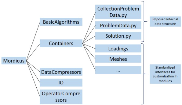
Fig. 2 Organization of the library
Data Model
The main feature of Mordicus is a data model adapted to reduced-order modeling.
It has been constructed to facilitate collaboration, by proposing three main classes
CollectionProblemData, ProblemData and Solution, supposed to be populated
and handle in the same fashion by all users:
CollectionProblemData: The meta structure containing the complete data model for a reduced-order model. See more details:Mordicus.Containers.CollectionProblemData().ProblemData: Containing a model for a physics problem: initial condition, loading, constitutive laws, solutions. See more details:Mordicus.Containers.ProblemData().Solution: Containing the size, snapshots and reduced coordinated of solutions. See more details:Mordicus.Containers.Solution().
These classes also contain numerous to iterate, modify and handle the data structure. We present a few important ones below:
CollectionProblemDatafunctions:DefineVariabilityAxes(): sets the axes of variability, can be strings for nonparametrized variability, or floats,SnapshotsIterator(): returns an iterator over snapshots of solutions of a given name,GetSnapshotsAtTimes(): returns an array containing all the snapshots of a given name, interpolated at a given time,CompressSolutions(): compress the snapshots of solutions of a given name against the corresponding reduced-order basis, and update to corresponding solution.reducedCoordinates.
Notice that the functions acting on solution object automatically iterate over all the problemDatas included in the collectionProblemData.
ProblemDatafunctions:UncompressSolution(): uncompress the reducedCoordinates of a solution of a given name, and update to corresponding solution.snapshots,GetLoadingsOfType(): returns all loadings of a specific type in a list,GetParameterAtTime(): returns the parameter value at a specitiy time (with time interpolation if needed).
Solutionfunctions:UncompressSnapshotAtTime(): uncompress the reducedCoordinates of the solution at a given time, and update to corresponding snapshots,GetTimeSequenceFromSnapshots(): returns the time sequence from the snapshots dictionary,ConvertReducedCoordinatesReducedOrderBasisAtTime(): converts the reducedSnapshot at a given time from the current reducedOrderBasis to a newReducedOrderBasis using a projectedReducedOrderBasis.
The data-model has also been thought to be agile and customizable, by allowing developers to propose other classes, in their applicative module, or variant classes of the ones contained in the subfolders of Containers (e.g. Loadings, Meshes, etc…).
Basic algorithms
Simple alogorithms are proposed, and can be used by any applicative module.
SVD: for computing truncated singular value decomposition of lower triangular matrices.ScikitLearnRegressor: contains examples for computing grid search cross validation and a customizable Gaussian Process Regressor using scikit-learn tools.Interpolation: contains efficient time Interpolation tool used in the Mordicus data model.