SnapshotsPODCompressionMeca

The use case can be downloaded here: exampleSnapshotsPODCompressionMeca

Features

In this tutorial, we consider a simple linear test case: a 3D elastic cube undergoing a constant pressure on a face, see Figure Fig. 3.

We illustrate how the Mordicus data structure is constructed and populated with high-fidelity data, then used to calculate a reduced order basis using the SnapshotPOD algorithm. Finally, the high-fidelity snapshots are reduced (compressed against the POD basis), and the accuracy of the compression is computed.

Commented code

List of imports required for this example:

from Mordicus.Containers import ProblemData as PD
from Mordicus.Containers import CollectionProblemData as CPD
from Mordicus.Containers import Solution as S
from Mordicus.DataCompressors import SnapshotPOD
from Mordicus.IO import StateIO as SIO
import numpy as np

Precomputed high-fidelity solutions for a given mechanical problem are read:

sol = SIO.LoadState("sol")

The Mordicus data structure, collectionProblemData, is declared. In this example, the variability of the problem is non-parametric: a string named “config” simply designs the different pre-computed high-fidelity problems. In this example, the solution is a displacement, noted “U”, in meters. Only one problem is considered here, and declared, with name “myProblem”.

collectionProblemData = CPD.CollectionProblemData()
collectionProblemData.DefineVariabilityAxes(('config',), (str,))
collectionProblemData.DefineQuantity("U", "displacement", "m")

problemData = PD.ProblemData("myProblem")

A Solution object is declared, with its number of compnents and number of nodes, associated to the quantity “U”, a primal variable. Its temporal sequence is read and affected, and the solution object is affected to the problem “myProblem”. This problem is itself affected to the collectionProblemData.

nbeOfComponents = 3
meshNumberOfNodes = 343

solution = S.Solution("U", meshNumberOfNodes, meshNumberOfNodes, primality = True)

outputTimeSequence = []
for time, snapshot in sol.items():
    solution.AddSnapshot(snapshot, time)
    outputTimeSequence.append(time)

problemData.AddSolution(solution)

collectionProblemData.AddProblemData(problemData, config="case-1")

The reduced order basis is computed using the SnapshotPOD algorithm, and is affected to the collectionProblemData for the “U” quantity.

reducedOrderBasis = SnapshotPOD.ComputeReducedOrderBasisFromCollectionProblemData(
    collectionProblemData, "U", 1.e-8
)
collectionProblemData.AddReducedOrderBasis("U", reducedOrderBasis)

The high-fidelity data is compressed against the POD basis.

collectionProblemData.CompressSolutions("U")

FInally, the accuracy of the compression is checked by recombining the general coordinates of the reduced solution (i.e. compressedSolution) with the POD basis, and computing the relative error with respect to the reference.

compressedSolution = solution.GetReducedCoordinates()

compressionErrors = []

for t in outputTimeSequence:

    reconstructedCompressedSolution = np.dot(compressedSolution[t], reducedOrderBasis)
    exactSolution = solution.GetSnapshot(t)
    norml2ExactSolution = np.linalg.norm(exactSolution)
    if norml2ExactSolution != 0:
        relError = np.linalg.norm(reconstructedCompressedSolution-exactSolution)/norml2ExactSolution
    else:
        relError = np.linalg.norm(reconstructedCompressedSolution-exactSolution)
    compressionErrors.append(relError)

Results

In Figure Fig. 3, the quality of the compression is illustrated by comparing the high-fidelity reference with the difference between this reference and the compressed snapshots (recombined with the POD modes).

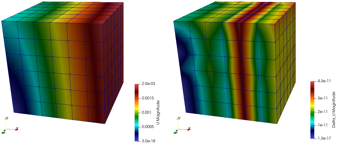
Fig. 3 Magnitude of the displacement at the last time step: (left) high-fidelity snapshots, (right) compressor error.

In Figure Fig. 4, the first two POD modes are illustrated.

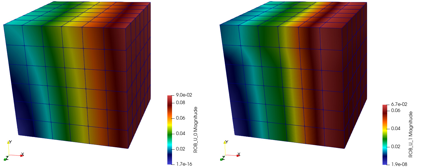
Fig. 4 POD modes: (left) first, (right) second.