Regression Thermal

The use case can be downloaded here: exampleRegressionThermal

The same features as in the tutorial SnapshotsPODCompressionThermal are illustrated, hence we only point out the differences here.

Features

In this tutorial, we consider a simple parametric linear thermal test case: a 2D square undergoing a convection heat flux in its 4 faces, see Figure Fig. 5. The test case is similar to the one considered in the tutorial tutorial SnapshotsPODCompressionThermal.

We illustrate how the Mordicus data structure is constructed and populated with high-fidelity data from 4 precomputed problems, then used to calculate a reduced order basis using the SnapshotPOD algorithm. Then, a regressor is trained to predict the generalized coordinates of the POD representation from the values of the parameters, and the offline generated data are saved on disk. Finally, the online stage is computed on a new parametric values.

Commented code: Offline stage

List of imports required for this example:

from Mordicus.Containers import ProblemData as PD
from Mordicus.Containers import CollectionProblemData as CPD
from Mordicus.Containers import Solution as S
from Mordicus.DataCompressors import SnapshotPOD
from Mordicus.OperatorCompressors import Regression
from Mordicus.IO import StateIO as SIO
import numpy as np

Precomputed high-fidelity solutions for 4 preomputed thermal problem are read:

sol = SIO.LoadState("sol")

The Mordicus data structure, collectionProblemData, is declared. In this example, the variability of the problem is parametric: two salar parameters ‘Text’ and ‘Tint are declared. In this example, the solution is a temperature field, noted “TP”, in degrees Celsius. Only one problem is considered here, and declared, with name “myProblem”.

solutionName = "TP"
nbeOfComponents = 1
numberOfNodes = 676
primality = True

collectionProblemData = CPD.CollectionProblemData()

collectionProblemData.AddVariabilityAxis('Text', float, quantities=('temperature', 'K'), description="this is Text")
collectionProblemData.AddVariabilityAxis('Tint', float, quantities=('temperature', 'K'), description="this is Tint")

collectionProblemData.DefineQuantity(solutionName, "Temperature", "Celsius")

For each of the 4 precomputed problems, a Solution object is declared, with its number of compnents and number of nodes, associated to the quantity “TP”, a primal variable. The solution object is affected to the problem “myProblem_i”. The time and parameter values are affected. Then, the considered problem is affected to the collectionProblemData.

parameters = [[100.0, 1000.0], [90.0, 1100.0], [110.0, 900.0], [105.0, 1050.0]]

for i in range(4):

    problemData = PD.ProblemData("myProblem_"+str(i))

    outputTimeSequence = []

    solution = S.Solution(
        solutionName=solutionName,
        nbeOfComponents=nbeOfComponents,
        numberOfNodes=numberOfNodes,
        primality=primality,
    )

    problemData.AddSolution(solution)

    for time, snapshot in sol[i].items():
        solution.AddSnapshot(snapshot, time)
        problemData.AddParameter(np.array(parameters[i] + [time]), time)
        outputTimeSequence.append(time)

    collectionProblemData.AddProblemData(problemData, Text=parameters[i][0], Tint=parameters[i][1])

The reduced order basis is computed using the SnapshotPOD algorithm, and is affected to the collectionProblemData for the “TP” quantity.

reducedOrderBasis = SnapshotPOD.ComputeReducedOrderBasisFromCollectionProblemData(
    collectionProblemData, solutionName, 1.e-2
)
collectionProblemData.AddReducedOrderBasis(solutionName, reducedOrderBasis)

The high-fidelity data is compressed against the POD basis.

collectionProblemData.CompressSolutions("TP")

A scikit-learn regressor is defined and affected to the “TP” solution name, and the regressor is trained.

from sklearn.gaussian_process.kernels import WhiteKernel, ConstantKernel, Matern
from sklearn.gaussian_process import GaussianProcessRegressor

kernel = ConstantKernel(constant_value=1.0, constant_value_bounds=(0.01, 10.0)) * Matern(length_scale=1., nu=2.5) + WhiteKernel(noise_level=1, noise_level_bounds=(1e-10, 1e0))

regressors = {"TP":GaussianProcessRegressor(kernel=kernel)}

paramGrids = {}
paramGrids["TP"] = {'kernel__k1__k1__constant_value':[0.1, 1.], 'kernel__k1__k2__length_scale': [1., 3., 10.], 'kernel__k2__noise_level': [1., 2.]}

Regression.CompressOperator(collectionProblemData, regressors, paramGrids)

The Mordicus data structure is then saved on disk. The snapshots are not saved, only their compressed representation in the form of general coordinates.

SIO.SaveState("collectionProblemData", collectionProblemData)

Commented code: Online stage

The Mordicus data structure is loaded from the disk.

collectionProblemData = SIO.LoadState("collectionProblemData")
reducedOrderBasis = collectionProblemData.GetReducedOrderBasis("TP")
onlineCompressionData = collectionProblemData.GetOperatorCompressionData("TP")

A problemData is declared for the online problem configuration (which consists, in this example, of the parameter values). The object onlineCompressionData, which has been read from collectionProblemData and contains the trained regressor, is affected to the problemData.

onlineProblemData = PD.ProblemData("Online")

OnlineTimeSequence = np.array(np.arange(200, 1001, 200), dtype=float)

for t in OnlineTimeSequence:
    onlineProblemData.AddParameter(np.array([95.0, 950.0] + [t]), t)

onlineProblemData.AddOnlineData(onlineCompressionData)

The online reduced problem is solved. In this example, it consists of evaluating the trained regressor.

reducedCoordinates = Regression.ComputeOnline(onlineProblemData, "TP")

The reference precomputed solution for this online confirguration is read, for comparison purposes.

ref = SIO.LoadState("ref")

FInally, the accuracy of the regression is checked by recombining the general coordinates of the reduced solution (i.e. compressedSolution) with the POD basis, and computing the relative error with respect to the reference.

compressionErrors = []
for t in reducedCoordinates.keys():
    reconstructedCompressedSolution = np.dot(reducedCoordinates[t], reducedOrderBasis)
    exactSolution = ref[t]
    norml2ExactSolution = np.linalg.norm(exactSolution)
    if norml2ExactSolution != 0:
        relError = np.linalg.norm(reconstructedCompressedSolution-exactSolution)/norml2ExactSolution
    else:
        relError = np.linalg.norm(reconstructedCompressedSolution-exactSolution)
    compressionErrors.append(relError)

Results

In Figure Fig. 7, the quality of the regression is illustrated by comparing the high-fidelity reference with the difference between this reference and the compressed snapshots (recombined with the POD modes).

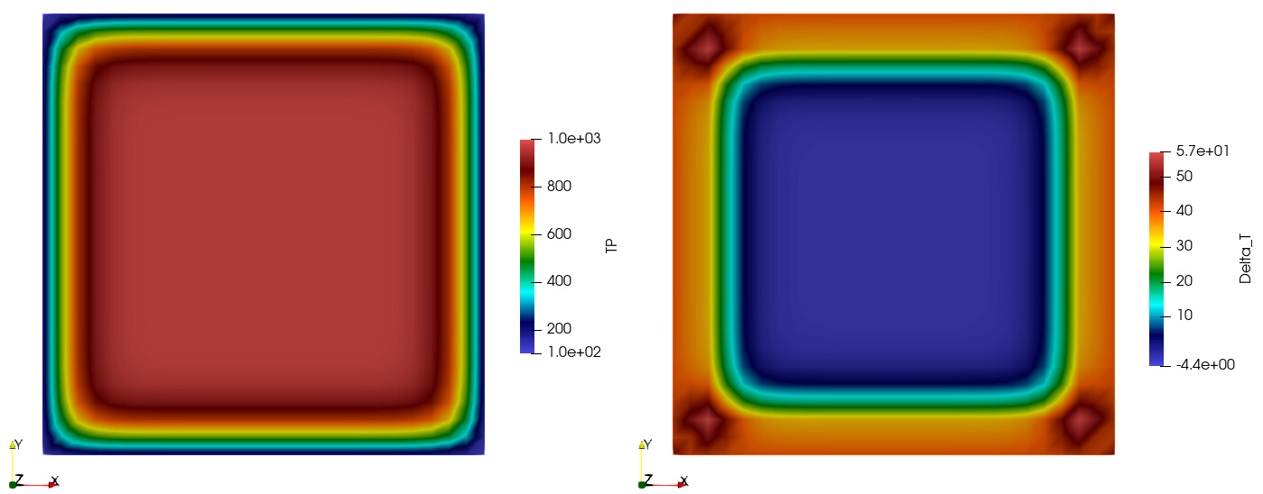
Fig. 7 Magnitude of the temperature at the last time step: (left) high-fidelity snapshots, (right) regression error.

In Figure Fig. 8, the first two POD modes are illustrated.

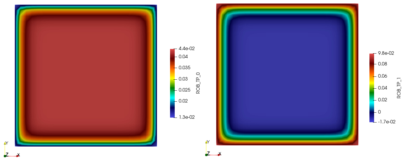
Fig. 8 POD modes: (left) first, (right) second.